Inputs	: 	Integer n_D indicating the size of training data 
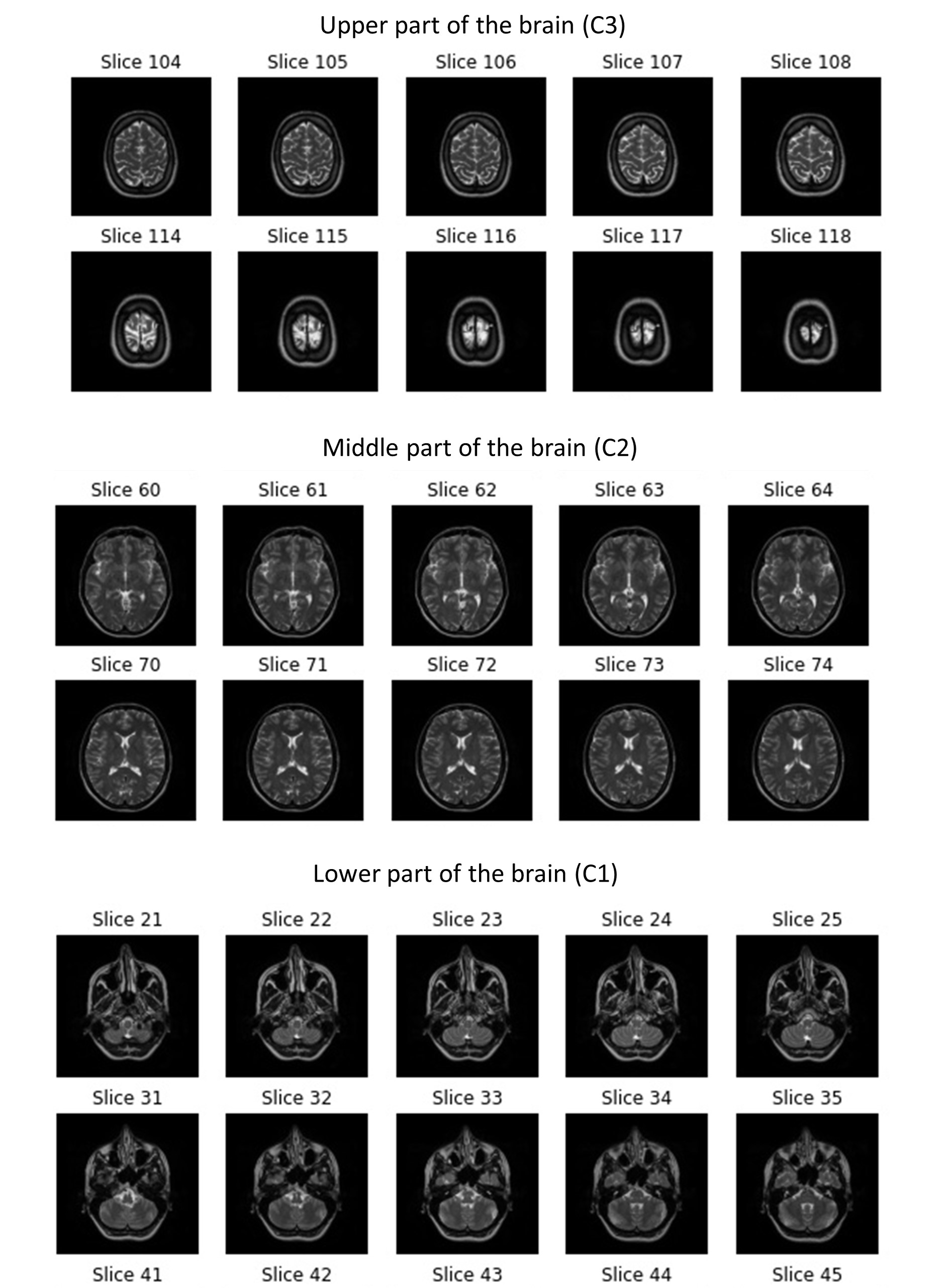
		List C containing the different classes {“C1”, “C2”, “C3”}
		String G representing the desired gender for the collection set: “M” for male or “F” for female
		Integer n_L_A and n_L_B representing the lower and upper bound for subject range, respectively

Outputs	: 	List D representing the sampled image slices for T2 and PD sequences

	Step 1: Re-defining the lower bound L_B of subject range
		if n_D < n_L_B then
		 n_L_B = n_D+n_L_A
		endif
	Step 2: Initializing necessary lists
		Initialize S to {“T2”, “PD”}, representing the list of MRI sequences
		Initialize D as empty two-dimensional list to store the sampled images from all sequences
		Initialize R as empty one-dimensional list to store randomly sampled image slice numbers.
	Step 3: Random sampling process based on stratified subject-wise splitting approach
		for each sequence s in S, do
		Open the directory of sequence s
		Get and open the directory of gender G within sequence s directory
		Initialize n_R to 0 for tracking the index in list R
		for each class c in C, do
			Initialize Y to the index of class c in C
			Get and open the directory of class c to retrieve list P of subject directories
			Initialize n_P to 0 for tracking the number of subjects processed
			for each subject p in P within the specified range 〖n_L〗_A and 〖n_L〗_B, do
				Step 3.1: Calculation of n_M for the count of sampled image slices
					if index of s=0, which indicates s is “T2”, then
						n_M = floor(n_D/n_L_B)+1
					else
						n_M = floor(n_D/n_L_B)
					endif
				Step 3.2: Calculation of n_T for the total number of image slices within subject p
					Get and open the directory of subject p to fetch list I consisting of image files
					Initialize n_T to 0
					for each image file i in I, do
						Increment n_T by 1
					endfor
				Step 3.3: Random selection of image slices from current subject p for sampling
					Randomly generate n_M numbers within the range of n_T 
					Add the generated randomized numbers to list R
				Step 4: Building the dataset of randomly sampled images
					Open the directory of subject p to fetch list I consisting of image files
					Initialize n_i to 0 for tracking the position of image file
					for each image file i in I, do
						Step 4.1: Selection of the correspondent image files for sampled slices
						if n_i is inside the list R[n_R], then
							Step 4.2: Feature extraction of selected image files
								Read current image file i and store the result to X
								Resize the shape of X to the desired image size of (224, 224, 3)
							Step 4.3: Storing extracted features and the label of sampled images
								Add X and Y of to D[index of sequence s in S]
						endif	
						Increment n_i by 1
					endfor
					Increment n_R by 1
				endfor
			endfor
		endfor
		Output D, where D[0] contains the sampled data for T2 and D[1] for PD sequence